Theory
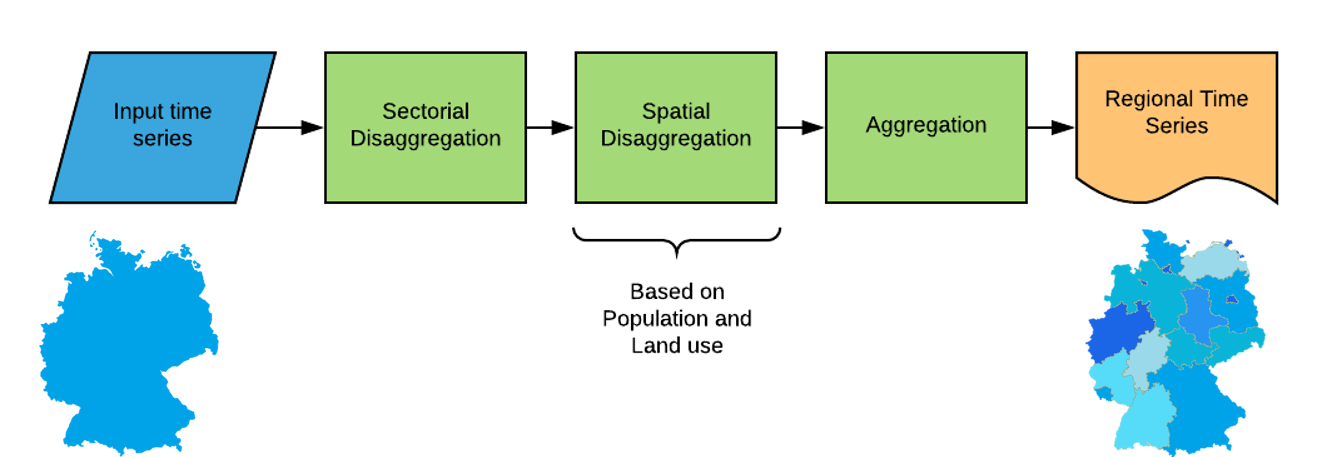
This chapters explains how the load time series are disaggregated spatially and according to sectors, then aggregated again according to the desired model regions.
Purpose
Load time series are widely available, but the published datasets are usually restricted to predefined spatial regions such as countries and their administrative subdivisions. The generate_load_timeseries() function takes the datasets which are available for these regions and disaggregate them according to a set of parameters, before aggregating them at a different spatial level. It is then possible to obtain time series for any region.
Description of lib.generate_intermediate_files.generate_load_timeseries
Inputs
The main inputs of this script are:
Load time series of the countries or regions to be disaggregated (hourly).
Shapefiles of the countries or regions to be disaggregated
Shapefiles of the regions of interest (subregions)
Assumptions (land use and sector correspondence)
Load profiles of the different sectors
Raster of the population and land use correspondent to the country or region
Sectoral disaggregation
The load is assumed to be perfectly divided into four distinct sectors (load sources):
Commercial
Industrial
Residential
Agricultural
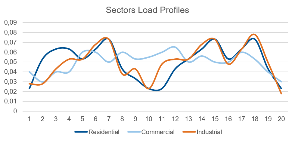
Sectoral load profiles
Sectoral load shares:
Region |
Industry |
Commerce |
Residential |
Agriculture |
|---|---|---|---|---|
A |
0.41% |
0.28% |
0.29% |
0.02% |
B |
0.31% |
0.30% |
0.38% |
0.01% |
C |
0.44% |
0.30% |
0.25% |
0.01% |
An hourly load profile for each sector has been predefined for one week, the same load profile is assumed to repeat over the year. These load profiles are scaled and normalized based on sectoral load shares for each region(assumed to be constant throughout the spatial scope), by multiplying the load profiles by their corresponding share and normalizing their hourly sum to be equal to 1.
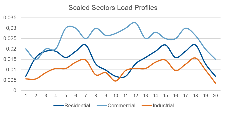
Scaled sectoral load profiles
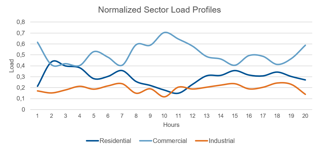
Normalized sectoral load profiles
Once the load profiles are normalized, we can multiply them with the actual load time series to obtain the load timeseries for each sector.
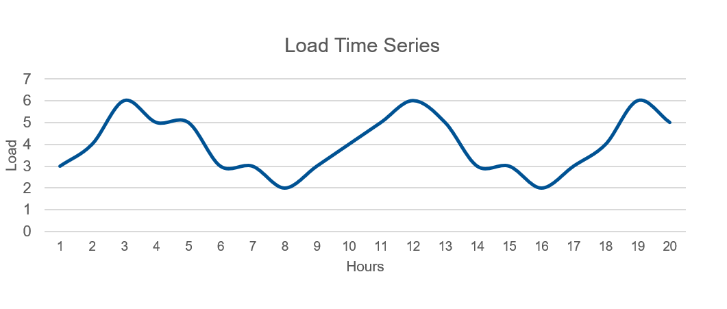
Load time series
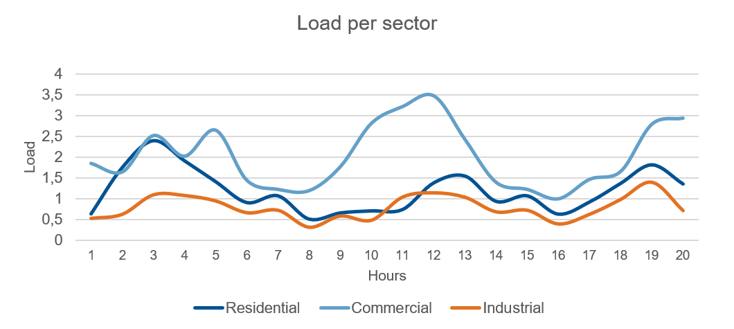
Sectoral load time series
Spatial disaggregation
The next step is the spatial disaggregation, based on the land use and population concentration rasters. First, each land-use type is assigned a sectoral load percentage corresponding to the load components of the land use category. Then, the population concentration raster is used to calculate the population of each pixel.
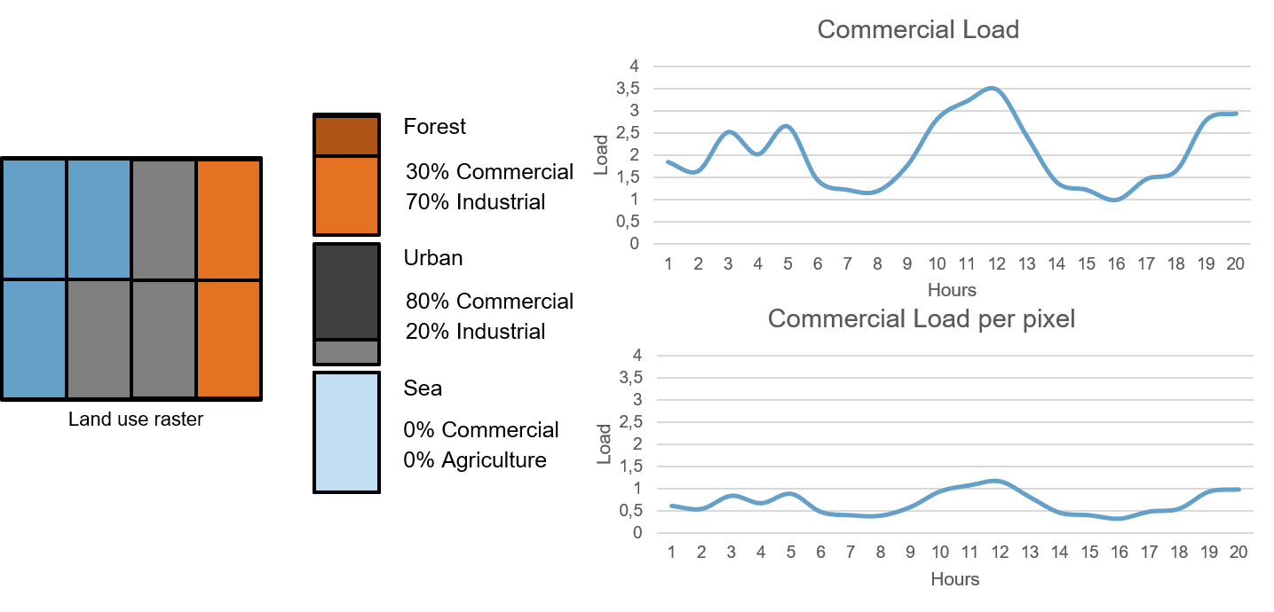
Example - Commerce sector spatial disaggregation
Counting the pixels, and land use occurrences inside of region for which the sectoral load timeseries has been calculated, the sectoral load for the Industry, commercial, and agricultural can be retrieved for each pixel of that region. Similarly, the residential load timeseries can be assigned to each pixel based on the population contained in the said pixel. The spatial disaggregation results in the assignment to every pixel inside a given region to be assigned a specific sectoral load timeseries.
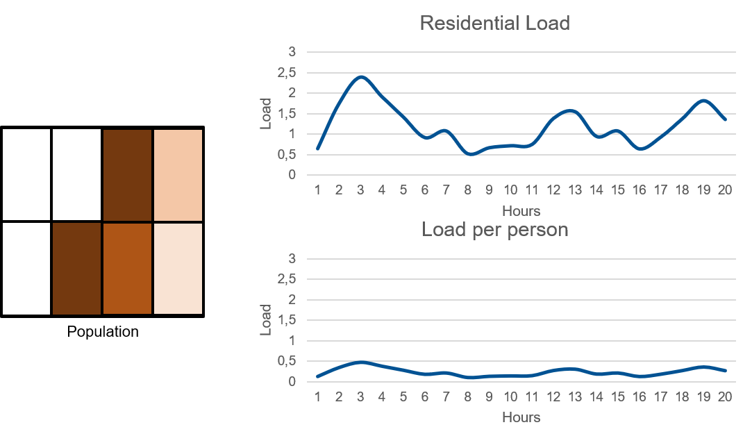
Example - Residential sector spatial disaggregation
Re-aggregation
The result of the sectoral and spatial disaggregation, performed in the first two sections can be used to retrieve the sectoral load timeseries and, therefore, the general load time series of any desired region by summing up the loads of every pixel contained within the region. If a subregion spans more than one region or country, it is divided into subregions restrained to each of those countries.